Solving nonlinearly separable classifications in a single layer neural network.
Recently, Ken Kurtz (my graduate advisor) and I figured out a unique solution to the famous limitation that single-layer neural networks cannot solve nonlinearly separable classifications. We published our findings in Neural Computation. This post is intended to provide a more introductory-level description of our solution. Read the paper for a more formal report!
Introduction
In an influential book published in 1969, Marvin Minsky and Seymour Papert proved that the conventional neural networks of the day could not solve nonlinearly separable (NLS) classifications.
Their conclusions spurred a decline in research on neural network models during the following two decades. It wasn't until the popularization of the backpropagation algorithm in the 1980s, which enabled models to solve NLS classifications through learning an additional layer of weights, that interest picked back up. But even after backprop, and after the advent of methods to train up deep networks, the conventional wisdom has been that the only way to solve a NLS classification is by adding layers of weights.
Recently, Ken Kurtz (my graduate advisor) and I figured out how you can solve NLS classifications with only a single layer of weights. In this post, I'll explain how!
What is a nonlinearly separable classification?
Nonlinearly separable classifications are most straightforwardly understood through contrast with linearly separable ones: if a classification is linearly separable, you can draw a line to separate the classes.
Below is an example of each. Imagine you are trying to discriminate between two classes, A and B, on the basis of two input dimensions (\(D_1\) and \(D_2\)):
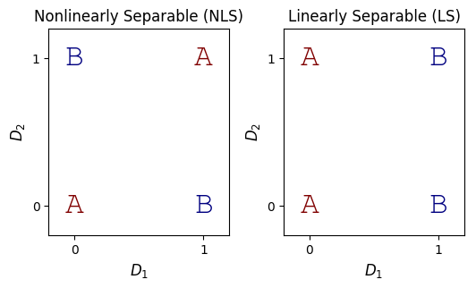
The NLS problem above is the ubiquitous Exclusive-Or (XOR) problem. Whereas you can easily separate the LS classes with a line, this task is not possible for the NLS problem.
Why can't a single layer network solve NLS classifications?
Drawing a line between the classes is like solving the classification with regression: the aim is to find the boundary the best separates the members of the two classes. And as it turns out, the traditional single-layer classifier is identical to a regression model:
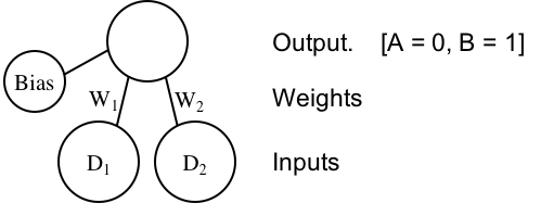
The network has two input units, \(D_1\) and \(D_2\), a bias unit, and a single output unit coding the response (say, 0 codes for A, and 1 codes for B). The inputs are connected to the outputs with weights, \(W_1\) and \(W_2\). So the model's output is given by:
$$ \begin{align} output & = D_1W_1 + D_2W_2 + bias \end{align} $$
Of course, that's also the canonical formula for regression. \(W_1\) and \(W_2\) are the slopes, and the bias is the intercept. The learning objective is to find the values of \(W_1\), \(W_2\), and bias that produce values of 0 for items in category A, and 1 for items in category B.
The above architecture is just a specific case of the more general multi-class network:
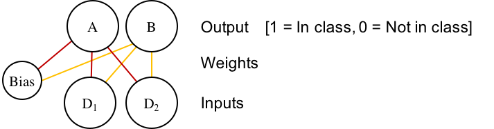
Where each class (again, A and B) gets its own output node. I've color-coded the weights so you can see how this is just two versions of the earlier network, put next to each other. So now output for each unit \(c\) is the sum of the product of each dimension \(D_k\) multiplied against the dimension's weight to the unit, \(W_{ck}\):
$$ \begin{align} output_c & = bias + \Sigma_k{D_k W_{ck}} \end{align} $$
In this more general case, it's useful to store the weights in an array to take advantage of matrix algebra to compute the output:
import numpy as np

                    # bias  D_1  D_2  # Correct Category
inputs = np.array([ [1,    0,   0],  # A
                    [1,    0,   1],  # A
                    [1,    1,   0],  # B
                    [1,    1,   1],  # B
    ])

# A perfect solution to the LS problem!
#                  A    B
wts = np.array([[ 1.0, 0.0], # bias
                [-1.0, 1.0], # W_1
                [ 0.0, 0.0], # W_2
            ])

output = np.dot(inputs, wts)

# output =
#      A   B
#   [[ 1.  0.]
#    [ 1.  0.]
#    [ 0.  1.]
#    [ 0.  1.]]
Note: for simplicity, bias is handled as an extra input unit that always has value 1. The real value of bias is specified in its weights.
But, again, this is identical to the simpler case, we're just doing it twice (once for A and once for B), and using matrix algebra for the computation in the equation above.
Anyway, the goal, of course, is to find values for \(W\) that correctly predict the category. But since this is akin to separating the categories with a line (which is what regression does), you'll never find useful values for an NLS problem: by definition, you cannot separate the classes with a line.
How to solve the NLS classification
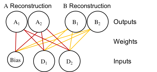
You definitely can't solve the NLS problem with any of the architectures above. So, the solution we came up with involves a re-envisioning of the problem, which is realized in a change to the architecture. Instead of the traditional perceptron architecture with dimensions-as-inputs and categories-as-outputs, we designed an autoassociator-based classifier:
Note: That architecture is actually a single-layer version of Ken's Divergent Autoencoder model, which is also very cool!
I've color-coded the weights so that it doesn't look like a tangled mess. Instead of having one output unit per category, the network has one output unit per category, per dimension. The output units are split into two, category-specific, channels, which is why we call it a "Divergent Autoassociator".
You could also imagine that network as two separate, regular autoassociators, which is formally the same (it just doesn't look divergent):
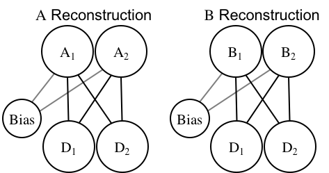
The network's goal is to "reconstruct" everything it sees in the correct category. So if \(D_1=0\) and \(D_2=1\) (i.e., input = [0,1]), and the network is told that belongs to category A, then the goal is for \(A_1=0\) and \(A_2=1\). The units on the opposite-category channel (\(B_1\) and \(B_2\)) are left alone.
Based on that learning objective, the network needs to learn weights that accurately reconstruct each category's items on the correct channel. This produces a network which learns how dimensions are correlated within each category, rather than a network which learns how dimensions predict categories.
Classification with the Divergent Autoassociator
Getting the model to classify things is about comparing the amount of error on each category channel. If, for example, the category A channel does a good job reconstructing [0, 1], and category B does a poor job, then the model will classify the item into category A.
Just to provide a sense of how the classification rule works, I calculated the optimal weights for the LS problem, and I copied over the network's output using those weights. Then, based on the output from each category, I computed the error and classification response.
import numpy as np

inputs = np.array([ [0,   0],
                    [0,   1],
                    [1,   0],
                    [1,   1] ])

# outputs copied from an optimal LS solution
output_A = np.array([[0,   0],
                    [0,   1],
                    [0,   0],
                    [0,   1] ])

output_B = np.array([[0.5,   0],
                    [0.5,   1],
                    [  1,   0],
                    [  1,   1] ])

error_A = np.sum((inputs - output_A)**2, axis = 1)
error_B = np.sum((inputs - output_B)**2, axis = 1)
classification = error_B < error_A
# classification =
#   [0 0 1 1]
The Single-Layer NLS Solution
So "solving" a classification in the Divergent Autoassociator involves finding a set of weights that allow each class to reconstruct its own members, but poorly reconstruct members of the other class. Here's how it's done:
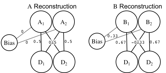
To prevent things from looking like a tangled mess, I've used the two-separate-autoassociators figure. But remember, this is just a single network! I've put the optimal weight values next to each weight.
Those weights result in the following outputs:
| Class | \(D_1\) | \(D_2\) | \(A_1\) | \(A_2\) | \(B_1\) | \(B_2\) |
|---|---|---|---|---|---|---|
| A | 0 | 0 | 0 | 0 | 0.33 | 0.33 |
| A | 1 | 1 | 1 | 1 | 0.67 | 0.67 |
| B | 0 | 1 | 0.5 | 0.5 | 0 | 1 |
| B | 1 | 0 | 0.5 | 0.5 | 1 | 0 |
You can see that the network has "solved" the NLS problem: items in category A are perfectly reconstructed by the A channel, but not in the B channel, and vice-versa. Here's the math for the final line: \(D_1\) = 1, \(D_2\) = 0
$$ \begin{align} A_1 = D_1 \cdot 0.5 + D_2 \cdot 0.5 + bias \\ = 1.0 \cdot 0.5 + 0.0 \cdot 0.5 + 0\\ = 0.5 + 0.0 + 0\\ = 0.5 \\ \\ A_2 = D_1 \cdot 0.5 + D_2 \cdot 0.5 + bias\\ = 1.0 \cdot 0.5 + 0.0 \cdot 0.5 + 0\\ = 0.5 + 0.0 + 0\\ = 0.5 \\ \end{align} $$
So the weights going to each category A output are identical. This shows that the network learned a key within-category regularity: \(D_1\) = \(D_2\). That is, you can always predict the value of \(D_1\) based on \(D_2\), because within category A the dimensions are positively correlated.
$$ \begin{align} B_1 = D_1 \cdot 0.67 + D_2 \cdot -0.33 + bias\\ = 1.0 \cdot 0.67 + 0.0 \cdot -0.33 + 0.33\\ = 0.67 + 0.0 + 0.33\\ = 1.0 \\ \\ B_2 = D_1 \cdot -0.33 + D_2 \cdot 0.67 + bias\\ = 1.0 \cdot -0.33 + 0.0 \cdot 0.67 + 0.33\\ = -0.33 + 0.0 + 0.33\\ = 0.0\\ \end{align} $$
The key difference in the category B channel is that the cross-dimension weights (e.g., going from \(D_1\) to \(B_2\)) are negative, showing that the network has learned the opposite pattern in category B: \(D_1\) will be the opposite of \(D_2\).
Summary
The Divergent Autoassociator solves the NLS classification without actually learning how to classify anything! Really, the model sidesteps the problem: first, it learns how to predict dimensions within each category, then it classifies items based on their consistency with what has been learned.
It doesn't do anything that differently from the traditional architecture: we didn't add a new computational step, we didn't add preprocessing, we didn't add a hidden layer. But by looking at the computational problem from a different angle, a new solution arises.
Explore it yourself!
Along with this post, I've written a couple simple python classes to explore learning in the traditional perceptron and divergent autoassociator models. They're probably not what you want to use for any rigorous study (they don't even classify things), but they're enough to explore what kinds of weight solutions are learned.
The classes can be found here. You can download them and import as a module like so:
import numpy as np
np.set_printoptions(precision = 2)

# import network objects
from single_layer_nets import perceptron
from single_layer_nets import autoassociator

# function to make 3d array printing prettier
from single_layer_nets import printattr

# define classes
NLS = dict( A = np.array([[0,0],[1,1]]),
            B = np.array([[0,1],[1,0]]),
            description = 'NLS')

LS = dict(  A = np.array([[0,0],[0,1]]),
            B = np.array([[1,0],[1,1]]),
            description = 'LS')

for categories in [LS, NLS]:
    print(' ----------- ' + categories['description'])
    print('Inputs:')
    print np.concatenate([categories['A'], categories['B']])

    for model in [perceptron, autoassociator]:

        # initialize network model
        net = model([categories['A'], categories['B']])
        net.train(1000)

        print('')
        print(net.model + ' output:')
        printattr(np.round(net.output, 2))

        print('')
        print(net.model + ' weights:')
        printattr(np.round(net.wts, 2))